Phylogenetic trees
Tudor-Stefan Cotet, Alexander Yermanos
10/06/2022
Source:vignettes/Phylogenetic trees.Rmd
Phylogenetic trees.Rmd1 Introduction
The Platypus family of packages are meant to provide potential pipelines and examples relevant to the broad field of computational immunology. The core set of functions can be found at https://github.com/alexyermanos/Platypus and examples of use can be found in the publications https://doi.org/10.1093/nargab/lqab023 and insert biorxiv database manuscript here
Stay tuned for updates https://twitter.com/AlexYermanos
To explore the clonal evolution across multiple clonotypes and samples (or at a whole-repertoire/global level), the Platypus ecosystem includes phylogenetic tree inference and plotting functions, with typical tree algorithms such as Neighbour-Joining, Maximum-Likelihood, and Maximum-Parsimony. Moreover, future Platypus updates will add ancestral sequence reconstruction utilities via the PHYLIP and IQ-TREE bioinformatics tools.
2. Loading the VGM
The output of the VDJ_GEX_matrix is the main object for all downstream functions in Platypus. We can create this directly into the R session by using the public data available on PlatypusDB. We will use the VDJ data of bone marrow plasma cells from five mice that were immunized with OVA (and the MPLA adjuvant) from Neumeier^, Yermanos^ et al 2022 PNAS.
## ── Attaching packages ─────────────────────────────────────── tidyverse 1.3.2 ──
## ✔ ggplot2 3.3.6     ✔ purrr   0.3.4
## ✔ tibble  3.1.8     ✔ dplyr   1.0.9
## ✔ tidyr   1.2.0     ✔ stringr 1.4.0
## ✔ readr   2.1.2     ✔ forcats 0.5.1
## ── Conflicts ────────────────────────────────────────── tidyverse_conflicts() ──
## ✖ dplyr::filter() masks stats::filter()
## ✖ dplyr::lag() masks stats::lag()## ggtree v3.4.1 For help: https://yulab-smu.top/treedata-book/
##
## If you use the ggtree package suite in published research, please cite
## the appropriate paper(s):
##
## Guangchuang Yu, David Smith, Huachen Zhu, Yi Guan, Tommy Tsan-Yuk Lam.
## ggtree: an R package for visualization and annotation of phylogenetic
## trees with their covariates and other associated data. Methods in
## Ecology and Evolution. 2017, 8(1):28-36. doi:10.1111/2041-210X.12628
##
## LG Wang, TTY Lam, S Xu, Z Dai, L Zhou, T Feng, P Guo, CW Dunn, BR
## Jones, T Bradley, H Zhu, Y Guan, Y Jiang, G Yu. treeio: an R package
## for phylogenetic tree input and output with richly annotated and
## associated data. Molecular Biology and Evolution. 2020, 37(2):599-603.
## doi: 10.1093/molbev/msz240
##
## S Xu, Z Dai, P Guo, X Fu, S Liu, L Zhou, W Tang, T Feng, M Chen, L
## Zhan, T Wu, E Hu, Y Jiang, X Bo, G Yu. ggtreeExtra: Compact
## visualization of richly annotated phylogenetic data. Molecular Biology
## and Evolution. 2021, 38(9):4039-4042. doi: 10.1093/molbev/msab166
##
## Attaching package: 'ggtree'
##
## The following object is masked from 'package:tidyr':
##
## expand
PlatypusDB_fetch(PlatypusDB.links = c("neumeier2021b//VDJmatrix"),
                                     load.to.enviroment = T, combine.objects = F)
## 2022-08-22 12:05:07: Starting download of neumeier2021b__VDJmatrix.RData...## [1] "neumeier2021b__VDJmatrix"
VDJ <- neumeier2021b__VDJmatrix[[1]]3. Creating phylogenetic trees via VDJ_phylogenetic_trees
1. Choosing the sequence type
The sequence type an be controlled via the sequence.type, as.nucleotide, and trimmed parameters in VDJ_phylogenetic_trees. For sequence.type, the following options are available: ‘VDJ’ for the VDJ full sequence, ‘VJ’ for the full VJ sequence, ‘VDJ.VJ’ for the combined VDJ/VJ sequences, ‘cdr3’ for the CDR3 region, ‘cdrh3’ for the CDRH3 region. To infer trees for protein sequences, use as.nucleotide = F. If trimmed is set to T, VDJ_phylogenetic_trees will look for the trimmed full sequences - ensure trim.and.align was set to T when obtaining your VGM using the VDJ_GEX_matrix function; else, trees will be inferred for the raw sequences.
We will next infer trees for the CDR3 sequences, with as.nucleotide set to T. We will only create 3 trees for a single sample (maximum.lineages = 3 which will subset the VDJ for the 3 most abundant clonotypes before creating the trees) for easier visualization. However, the usual output of VDJ_phylogenetic_trees is a nested list of tidytree objects (per sample, per clonotype), whereas the output of VDJ_phylogenetic_trees_plot is a list of intraclonal trees for each clonotype/lineage obtained from VDJ_phylogenetic_trees.
We will also set the maximum.sequences parameter to 20 to only obtain trees with a maximum of 20 sequences (the top 20 most frequent sequences per clonotype) and minimum.sequences to 1 (avoiding singletons). Moreover, we will set include.germline to F (otherwise VDJ_phylogenetic_trees will look for germlines/10x references in the VDJ and VJ_trimmed_ref columns).
s1_subset <- VDJ[VDJ$sample_id == 's1',]
p <- s1_subset %>% VDJ_phylogenetic_trees(sequence.type = 'cdr3',
                                     as.nucleotide = T,
                                     trimmed = F,
                                     minimum.sequences = 3,
                                     maximum.sequences = 20,
                                     maximum.lineages = 3,
                                     include.germline = F) %>%
                   VDJ_phylogenetic_trees_plot()

cowplot::plot_grid(plotlist = p)
We can see how the first clonotype was filtered out, as it had fewer sequences that the minimum in minimum.sequences.
2. Phylogenetic tree algorithms
The following tree inference algorithms are supported by VDJ_phylogenetic_trees: Neighbour-Joining via the ape package (tree.algorithm = ‘nj’), Maximum-Likelihood via the phangorn package (tree.algorithm = ‘ml’), and Maximum-Parsimony via the phangorn package (tree.algorithm = ‘mp’).
Neighbour-joining trees
#Neighbour-joining trees via the ape package
s1_subset <- VDJ[VDJ$sample_id == 's1',]
p <- s1_subset %>% VDJ_phylogenetic_trees(sequence.type = 'cdr3',
                                     as.nucleotide = T,
                                     trimmed = F,
                                     minimum.sequences = 3,
                                     maximum.sequences = 20,
                                     maximum.lineages = 3,
                                     include.germline = F,
                                     tree.algorithm = 'nj') %>%
                   VDJ_phylogenetic_trees_plot()

cowplot::plot_grid(plotlist = p)
Maximum-likelihood trees
#Maximum-likelihood trees via the phangorn package
s1_subset <- VDJ[VDJ$sample_id == 's1',]
p <- s1_subset %>% VDJ_phylogenetic_trees(sequence.type = 'cdr3',
                                     as.nucleotide = T,
                                     trimmed = F,
                                     minimum.sequences = 3,
                                     maximum.sequences = 20,
                                     maximum.lineages = 3,
                                     include.germline = F,
                                     tree.algorithm = 'ml') %>%
                   VDJ_phylogenetic_trees_plot()

cowplot::plot_grid(plotlist = p)
Maximum parsimony trees
#Maximum parsimony trees via the phangorn package
s1_subset <- VDJ[VDJ$sample_id == 's1',]
p <- s1_subset %>% VDJ_phylogenetic_trees(sequence.type = 'cdr3',
                                     as.nucleotide = T,
                                     trimmed = F,
                                     minimum.sequences = 3,
                                     maximum.sequences = 20,
                                     maximum.lineages = 3,
                                     include.germline = F,
                                     tree.algorithm = 'mp') %>%
                   VDJ_phylogenetic_trees_plot()

cowplot::plot_grid(plotlist = p)3. Per-repertoire/global trees
VDJ_phylogentic_trees can also be used to obtain per-repertoire or global trees, by combining all sequences available across a single repertoire/across all repertoires. This can be customized via the tree.level parameter, which defaults to ‘intraclonal’ (per clonotype trees). Setting tree.level to ‘combine.first.trees’ will combine the n most abundant clonotypes in a single sample, as determined by the parameter n.trees.combined. The other option for tree.level is ‘global.clonotype’ which will combine trees in the same clonotype, irrespective of samples (useful when global clonotypes are defined across multiple repertoire, via VDJ_call_enclone).
We will combine the first 3 trees in sample s1 by setting tree.level to ‘combine.first.trees’ and n.trees.combined = 3. We will also set maximum.sequences to NULL to allow trees to be inferred from all sequences available.
s1_subset <- VDJ[VDJ$sample_id == 's1',]
s1_subset %>% VDJ_phylogenetic_trees(sequence.type = 'cdr3',
                                         as.nucleotide = T,
                                         trimmed = F,
                                         maximum.sequences = NULL,
                                         include.germline = F,
                                         minimum.sequences = 0,
                                         tree.algorithm = 'nj',
                                         tree.level = 'combine.first.trees',
                                         n.trees.combined = 3
                                         ) %>%
                   VDJ_phylogenetic_trees_plot()
## [[1]]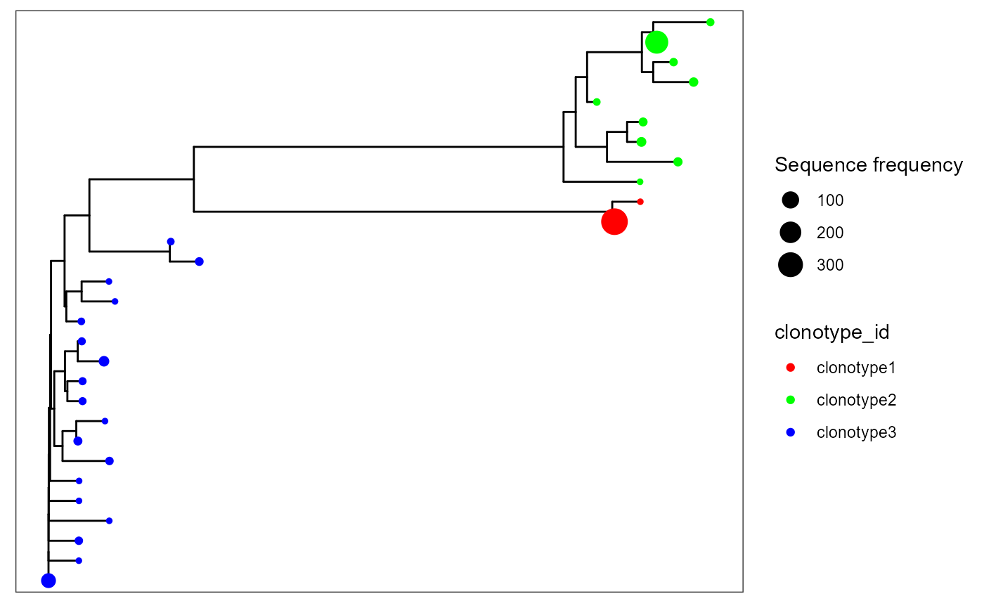
4. Custom tree plots via VDJ_phylogenetic_trees_plot
To add new features to your trees (from the VDJ matrix), use the additional.feature.columns parameter. These new features can be used for more flexible plotting. For example, additional.feature.columns = c(‘VDJ_vgene’, ‘VDJ_jgene’) will add the respective V and J genes per unique sequence.
Change the tip colors
You can change tree tip colors via the color.by parameter in VDJ_phylogenetic_trees_plot.
#Trees with tips colored by V gene.
s1_subset <- VDJ[VDJ$sample_id == 's1',]
s1_subset %>% VDJ_phylogenetic_trees(sequence.type = 'cdr3',
                                         as.nucleotide = T,
                                         trimmed = F,
                                         maximum.sequences = NULL,
                                         include.germline = F,
                                         minimum.sequences = 0,
                                         tree.algorithm = 'nj',
                                         tree.level = 'combine.first.trees',
                                         n.trees.combined = 3,
                                         additional.feature.columns = 'VDJ_vgene'
                                         ) %>%
              VDJ_phylogenetic_trees_plot(color.by = 'VDJ_vgene')
## [[1]]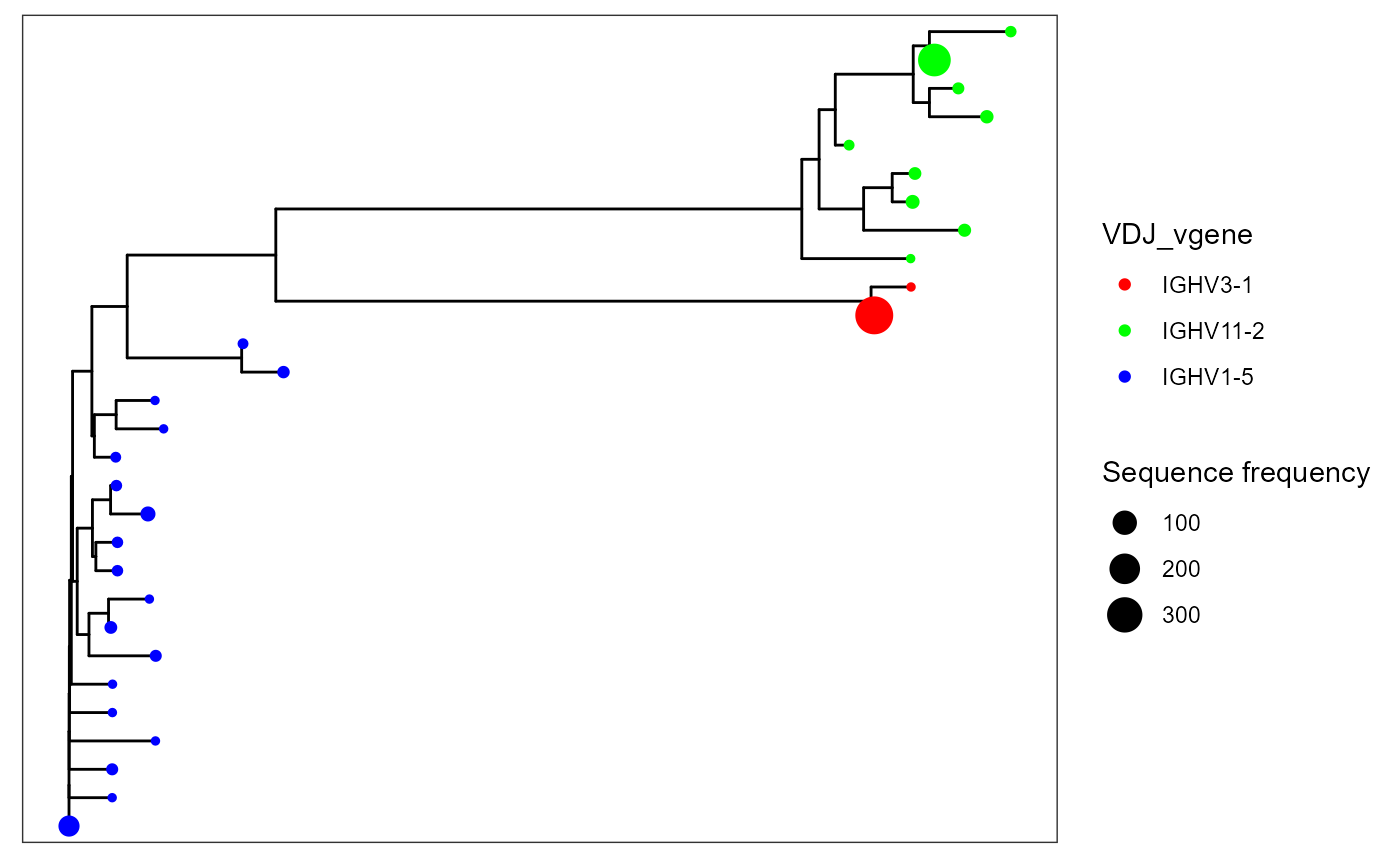
Moreover, you can specify a list of custom colors in the specific.leaf.colors parameter.
#Trees with tips colored by V gene.
s1_subset <- VDJ[VDJ$sample_id == 's1',]
s1_subset %>% VDJ_phylogenetic_trees(sequence.type = 'cdr3',
                                         as.nucleotide = T,
                                         trimmed = F,
                                         maximum.sequences = NULL,
                                         include.germline = F,
                                         minimum.sequences = 0,
                                         tree.algorithm = 'nj',
                                         tree.level = 'combine.first.trees',
                                         n.trees.combined = 3,
                                         additional.feature.columns = 'VDJ_vgene'
                                         ) %>%
              VDJ_phylogenetic_trees_plot(color.by = 'VDJ_vgene',
                                           specific.leaf.colors = list('IGHV3-1' = 'yellow','IGHV11-2' = 'orange', 'IGHV1-5' = 'red'))
## [[1]]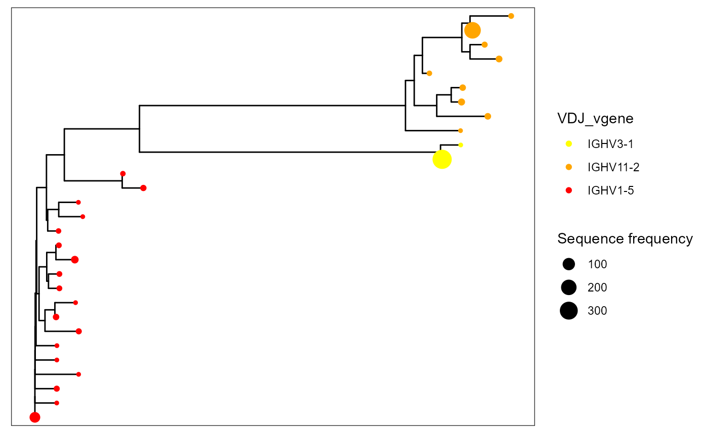
5. Version information
## R version 4.2.1 (2022-06-23 ucrt)
## Platform: x86_64-w64-mingw32/x64 (64-bit)
## Running under: Windows 10 x64 (build 19044)
##
## Matrix products: default
##
## locale:
## [1] LC_COLLATE=German_Germany.utf8  LC_CTYPE=German_Germany.utf8
## [3] LC_MONETARY=German_Germany.utf8 LC_NUMERIC=C
## [5] LC_TIME=German_Germany.utf8
##
## attached base packages:
## [1] stats     graphics  grDevices utils     datasets  methods   base
##
## other attached packages:
##  [1] ggtree_3.4.1    forcats_0.5.1   stringr_1.4.0   dplyr_1.0.9
##  [5] purrr_0.3.4     readr_2.1.2     tidyr_1.2.0     tibble_3.1.8
##  [9] ggplot2_3.3.6   tidyverse_1.3.2 Platypus_3.4.1
##
## loaded via a namespace (and not attached):
##  [1] nlme_3.1-157        fs_1.5.2            lubridate_1.8.0
##  [4] httr_1.4.3          rprojroot_2.0.3     tools_4.2.1
##  [7] backports_1.4.1     bslib_0.4.0         utf8_1.2.2
## [10] R6_2.5.1            DBI_1.1.3           lazyeval_0.2.2
## [13] colorspace_2.0-3    withr_2.5.0         tidyselect_1.1.2
## [16] curl_4.3.2          compiler_4.2.1      textshaping_0.3.6
## [19] cli_3.3.0           rvest_1.0.2         xml2_1.3.3
## [22] desc_1.4.1          labeling_0.4.2      sass_0.4.2
## [25] scales_1.2.0        pkgdown_2.0.6       systemfonts_1.0.4
## [28] digest_0.6.29       yulab.utils_0.0.5   rmarkdown_2.14
## [31] stringdist_0.9.8    pkgconfig_2.0.3     htmltools_0.5.3
## [34] highr_0.9           dbplyr_2.2.1        fastmap_1.1.0
## [37] rlang_1.0.4         readxl_1.4.0        rstudioapi_0.13
## [40] farver_2.1.1        gridGraphics_0.5-1  jquerylib_0.1.4
## [43] generics_0.1.3      jsonlite_1.8.0      googlesheets4_1.0.0
## [46] magrittr_2.0.3      ggplotify_0.1.0     patchwork_1.1.1
## [49] Rcpp_1.0.9          munsell_0.5.0       fansi_1.0.3
## [52] ape_5.6-2           lifecycle_1.0.1     stringi_1.7.8
## [55] yaml_2.3.5          grid_4.2.1          parallel_4.2.1
## [58] crayon_1.5.1        lattice_0.20-45     haven_2.5.0
## [61] cowplot_1.1.1       hms_1.1.1           knitr_1.39
## [64] pillar_1.8.0        codetools_0.2-18    reprex_2.0.1
## [67] glue_1.6.2          evaluate_0.15       ggfun_0.0.6
## [70] modelr_0.1.8        vctrs_0.4.1         treeio_1.20.1
## [73] tzdb_0.3.0          foreach_1.5.2       cellranger_1.1.0
## [76] gtable_0.3.0        assertthat_0.2.1    cachem_1.0.6
## [79] xfun_0.31           broom_1.0.0         tidytree_0.3.9
## [82] ragg_1.2.2          googledrive_2.0.0   gargle_1.2.0
## [85] iterators_1.0.14    aplot_0.1.6         memoise_2.0.1
## [88] ellipsis_0.3.2